AI-era DCI: Beyond the chip, compete as a network. Is there a China play?

Under the Scaling Law, LLM parameter counts keep exploding and multi-turn dialogue demands ever-growing state storage. Single cards no longer have enough compute or HBM to handle cutting-edge training and inference. AI workloads therefore must run on ultra-scale clusters coordinated across massive fleets of xPUs.

What stitches single cards into clusters and thousands of heterogeneous chips inside and across clusters into one logical machine is the AI interconnect fabric. It turns many chips into a coherent system through high-speed links and networked orchestration.

The tech roadmaps of GPGPU and AI ASIC vendors over recent years show the pivot from chasing single-die peak FLOPS to engineering at cluster scale. The spotlight has shifted from chip specs to system-level throughput and reliability.

Today, training is sharded across thousands to tens of thousands of xPUs, with every step and gradient update interleaved by heavy collective communications. In synchronous parallelism, all cards must wait for the slowest link before moving to the next step, creating a classic bottleneck. This ‘barrel effect’ makes the interconnect as critical as the accelerators themselves.

China lagged in the single-die era. But in the era of AI interconnects that prize high bandwidth and low latency, Jensen Huang has noted that single-die weaknesses can be mitigated via networking, which aligns with Huawei’s strengths. Huawei has its own custom UB protocol, in-house switches, and powerful interconnect capabilities that close system-level gaps.

Dolphin Research has conducted a series of studies to understand the layering of AI interconnects. This piece starts from first principles to build an intuitive framework.

1) How are AI data centers wired and connected? What are the practical boundaries and scopes at each layer?

2) What core concepts and building blocks does the fabric comprise? How do these elements interact in real deployments?

I. What is a network connection?

Building a data center requires XPU fleets such as GPUs and CPUs, storage, NICs, and switches. Connections tie these disparate devices via fiber and copper into a high-speed, information-rich network. The goal is consistent, high-throughput, low-latency data exchange across many tiers.

The core tenets are not fundamentally different from traditional interconnects. But tighter coupling and higher speed/throughput raise the bar for engineering, power, and thermal design, pushing systems toward more integrated solutions.

Let’s look at the AI networking stack used by $NVIDIA(NVDA.US) & $AMD(AMD.US), which is broadly representative. Physically, by distance from inside out, it breaks into three layers:

1) Within a tray — interconnects between the CPU and nearby devices; 2) Within and across racks — interconnects among xPUs on and across trays; 3) Data center-to-data center interconnects for long-haul links.

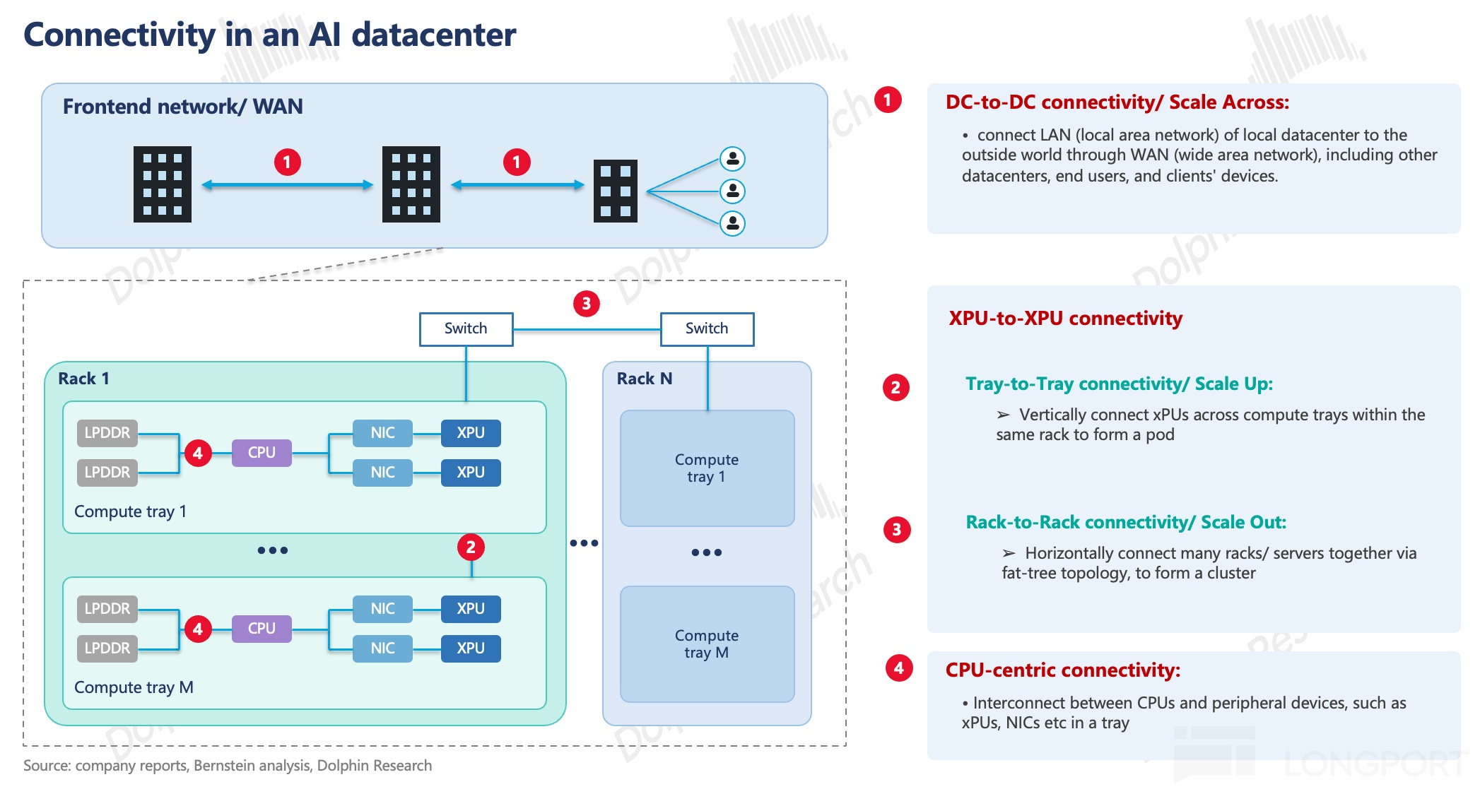
Think of an AI DC as a campus executing a massive, time-critical project (AI workloads). The campus has many office buildings (racks), each with multiple compute floors (compute trays) and scheduling floors (switch trays with embedded switch ASICs). Compute floors host engineers (xPUs) who do the heavy lifting, while the project managers (CPUs) assign tasks, pull data, and interface externally, and the reception (NIC) handles ingress/egress.

Work is split into tens of thousands of pieces and runs in parallel. Ultimately, ‘who talks to whom, and how quickly they align’ determines the overall timeline and throughput for completion.

1) Within a tray — CPU-to-peripheral interconnects: This layer coordinates CPU communications with xPUs, NICs, and other devices. Physically, it is implemented via PCB traces, measured in centimeters, with ultra-low latency in the nanoseconds range. Functionally, it handles internal/external data movement and dispatches workloads to xPUs.

2) Within and across racks — xPU-to-xPU interconnects: This is the compute brain of the AI era, the layer where the actual ‘engineers’ must be tightly networked to behave like one ‘super engineer’. It is evolving the fastest and is the primary focus of this piece, as performance here sets cluster limits.

- Tray-to-tray (Scale-up): Even if multiple engineers sit on the same floor, they do not talk point-to-point. Instead, each sends information to the scheduling floor (switch tray), which then forwards to the intended recipients. This is because communications are often many-to-many across dozens or hundreds of participants, and relaying via people would add delay.

Centralized forwarding avoids multi-hop human relays and minimizes latency at short reach. In other words, inside a tray, even adjacent GPUs have no direct links and rely on the scheduling layer for delivery.

Physically, signals leave the xPU via PCB out of the tray, then traverse copper to the switch layer. As xPU counts scale, this link strategy keeps evolving. Copper is predominant here today, and its physical limits shape engineer–scheduler–engineer communication capabilities.

Note that using rack boundaries to demarcate Scale-Up vs. Scale-Out by physical distance is not strictly accurate, though it is intuitive. NVIDIA’s Rubin Ultra extends Scale-Up beyond a rack, blurring the line. The true distinction lies in protocol semantics and how memory is addressed.

- Scale-Up is instruction-level load/store access, where the switch ASIC fetches by address (memory semantics). This yields lower latency and direct addressing of remote memory.

- Scale-Out resembles parcel delivery. Content must be encapsulated, labeled, and transported, then acknowledged upon receipt (message semantics with protocol encapsulation and confirmation).

In most common topologies (excluding Huawei), Scale-Up domains typically include only xPUs. Other rack components like CPUs and storage sit outside that domain and communicate via message semantics rather than direct loads/stores.

For example, a CPU reaching another tray’s CPU uses the message path akin to one server talking to another: CPU → PCIe → NIC/DPU → switch → remote DPU → PCIe → CPU. This is effectively Scale-Out even if both are in the same rack.

- Rack-to-rack (Scale-out): Multiple buildings (racks) are chained into a coordinated training cluster (Pod/SuperPod). Cross-building traffic does not go through the scheduling floor and instead flows from xPUs to NICs for egress.

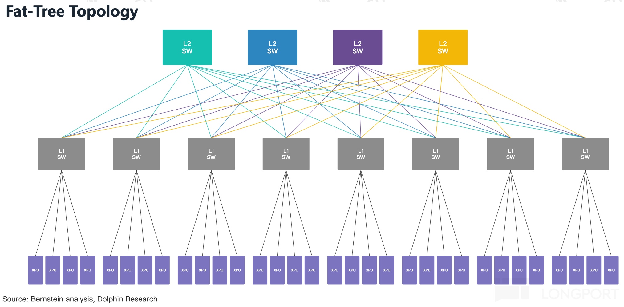
It is then forwarded through Ethernet switches (the campus mailroom) in hierarchical topologies like two- or three-tier fat trees, relying on optical modules at 400G, 800G, and 1.6T. The core challenges shift from ‘how fast to send’ to congestion control, TCO, and coordinating tens of thousands of accelerators.

3) Data center interconnect (Scale-across): Long-haul optical networking links multiple campuses or regions to support cross-region workload distribution, data replication, and end-user access. This layer relies on coherent DWDM optics for spectral efficiency and long reach.

Distances span tens to hundreds of kilometers, with per-wavelength bandwidth at 400G–800G and a roadmap to 1.6T/3.2T. Because it carries regional traffic rather than synchronous, step-critical training, higher latency is tolerable at this layer.

II. Network connections: key hardware and how it works

We have outlined ‘who talks to whom’. Next is ‘with what and how’. The core splits into two buckets: hardware such as PCBs, switches, NICs, optical modules, copper cables, and fiber, and software, namely protocols and ecosystems that define semantics and scale.

We start with hardware since shipments and installed base under each protocol define the hard power of an interconnect ecosystem. Adoption determines which standard wins in practice.

1) Hardware: device shipments and share under each protocol are the hard-power metrics of the ecosystem

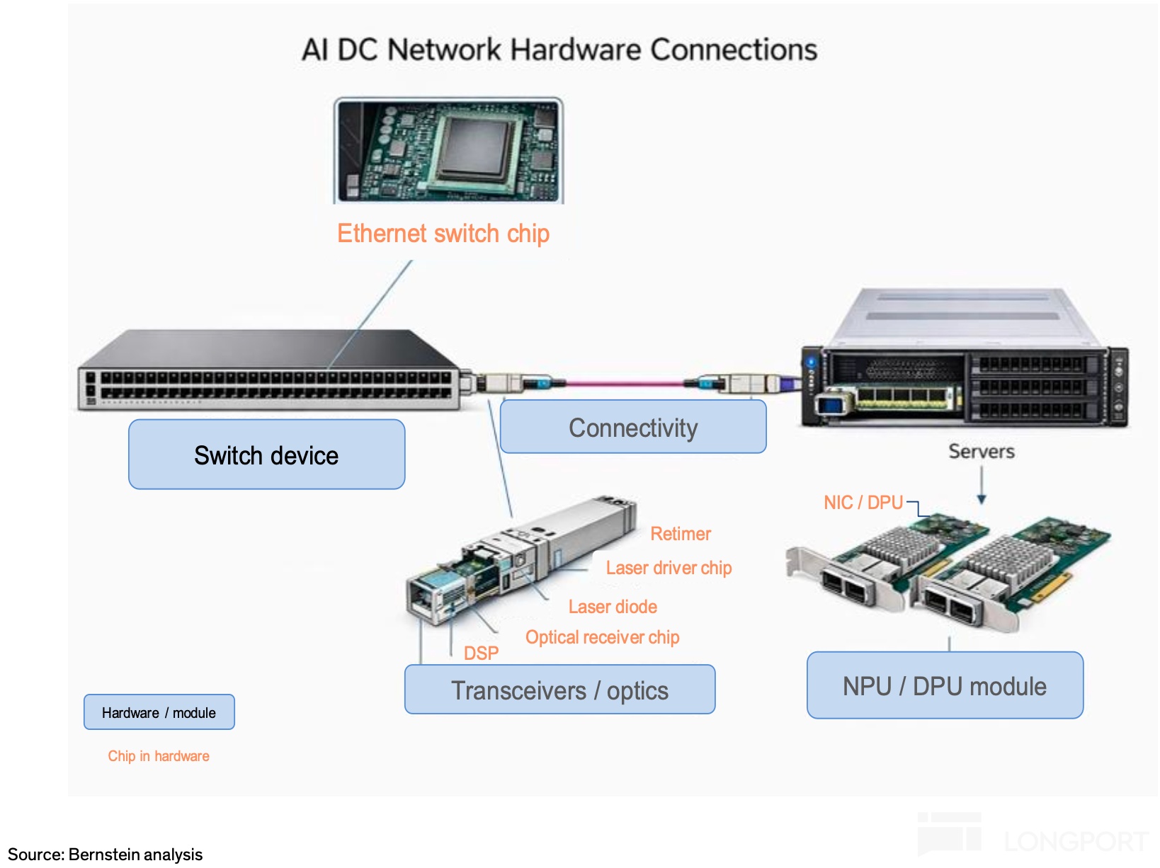
Hardware roughly clusters into three module classes: switches, connectivity/optics, and NICs/DPUs. Each module centers on dedicated silicon that provides bandwidth, signal integrity, and compute offload required by AI clusters.

a) Switches: high value-add across the chain, high GPM

Switches form the network and are the core aggregation/forwarding gear in AIDC, scheduling traffic among xPUs like a campus mailroom. The switch ASIC dictates chassis throughput, latency, and power, directly shaping system performance.

Aggregate bandwidth is a product of port count and per-port speed. Leading platforms support 51.2T today and are moving to 102.4T, aligning to 400G, 800G, and 1.6T link speeds per port in the line cards.

In common fat-tree topologies, switches are layered into ToR/Leaf, Spine, and Super-Spine in three-tier designs. ToR/Leaf sits at the top of the rack and connects down to server NICs, being the only tier directly linked to xPUs, while upper tiers interconnect switches and scale out the fabric.

b) Optics/connectivity

• Optical modules: high-value chips with high GPM; module competition is intense

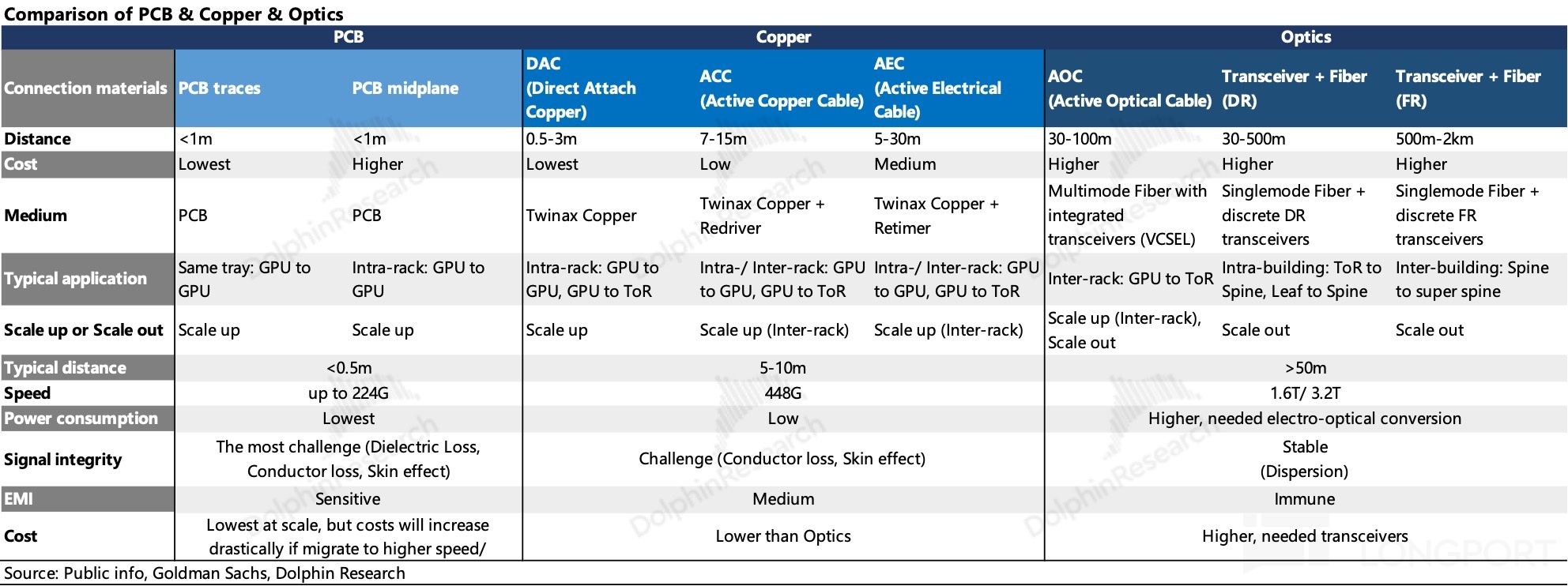
Optical modules perform bidirectional E/O and O/E conversion between switch/NIC electrical interfaces and optical links. They act as ‘translators’ in the data path and are indispensable in Scale-Out, while increasingly extending Scale-Up beyond copper’s reach.

As links move to 800G, 1.6T, and even 3.2T, power, thermal, and signal integrity become key bottlenecks. These pressures accelerate the shift from pluggables (dominant at 400G/800G) to LPO and CPO. For more, cf. the linked pieces on technology and supply chain.

• Transmission media: mid value-add, heavy competition

Copper interconnects are valued for low power, cost efficiency, and reliability, but signal quality degrades quickly with longer reach or higher speeds. Copper is typically limited to ≤30 meters, confining it largely to in-rack Scale-Up use. Notably, NVIDIA’s Rubin Ultra introduces PCB-based backplanes to replace copper cables for in-rack Scale-Up.

Optical links provide high bandwidth and long reach with lower attenuation and scale to Tbps, making them the mainstream for rack-to-rack Scale-Out. They underpin the spine layers where most aggregation occurs.

c) NIC/DPU

The NIC is the network endpoint on each node, connected to xPUs/CPUs via PCIe or proprietary links. It sends/receives packets to/from switches and sets the practical communication efficiency on Scale-Out paths.

NICs are rapidly evolving into SmartNICs with programmable logic to offload non-core compute tasks from CPUs, freeing CPU cycles for AI orchestration and scheduling. DPUs go further by taking over networking, storage, and security functions as a converged data-plane processor.

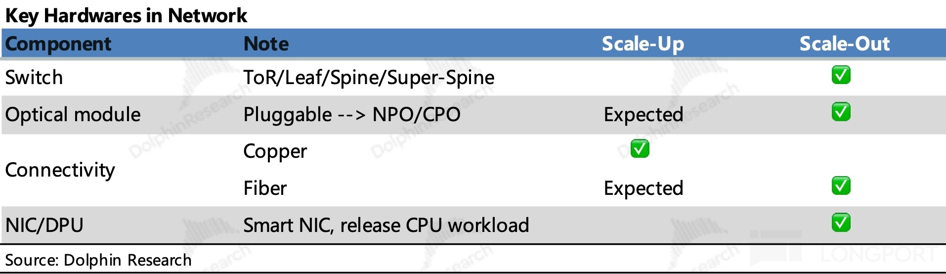
2) How does the hardware operate?

Each component plays a specific role in the AI network. The next question is how they cooperate to execute AI workloads at system scale. We explain this by following the signal’s path through the stack to see how the pieces form a cohesive system.

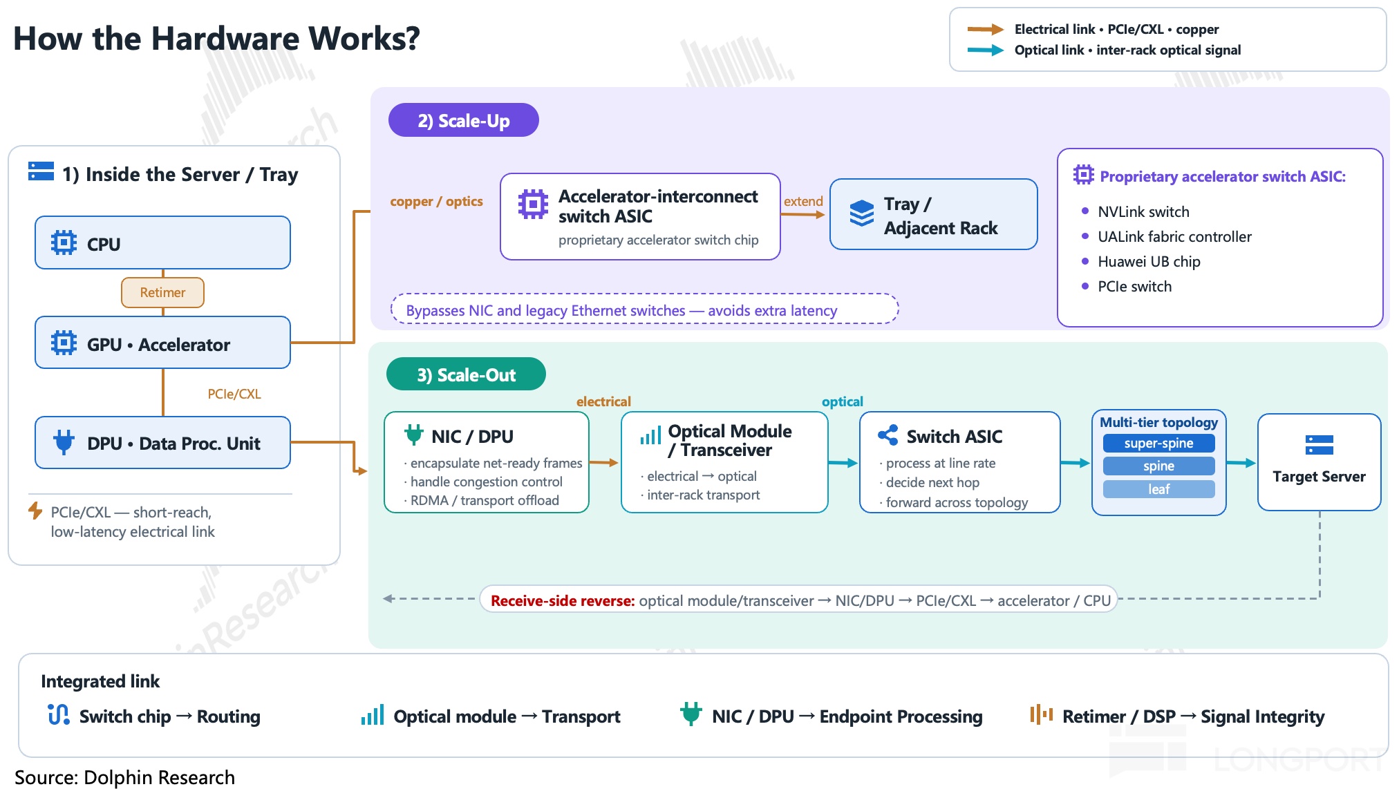
The overall flow is illustrated below, from node internals to rack-scale and beyond. The same principles apply whether the payload is training, inference, or data replication.

a) Inside the node

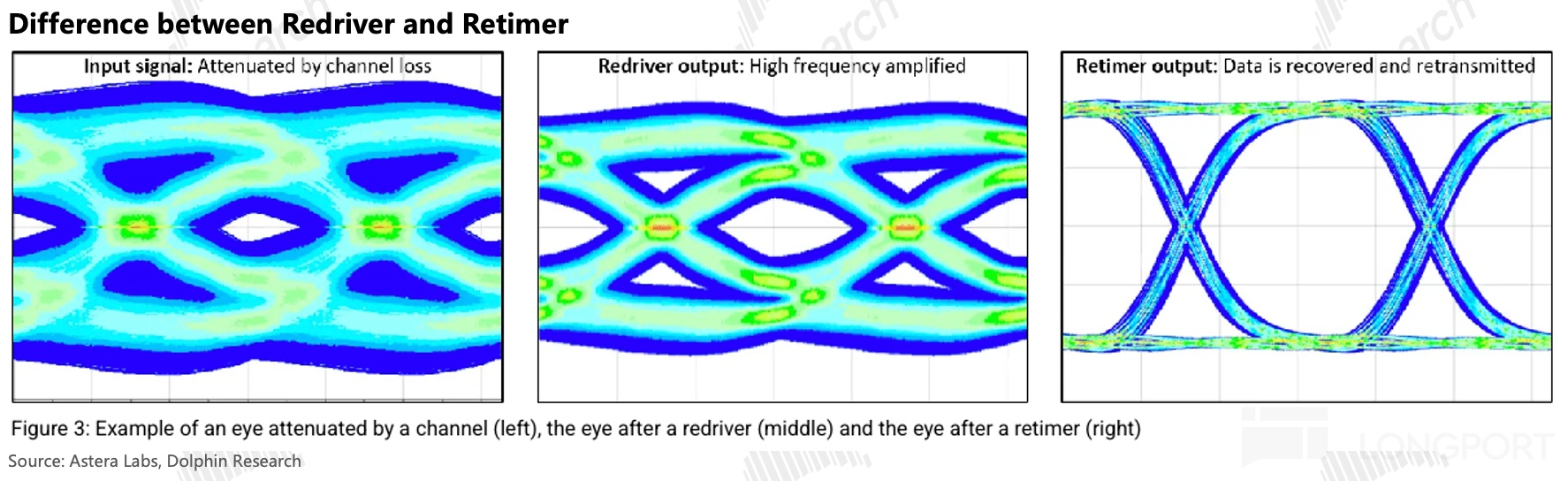
Inside a server, CPUs, GPUs, and NICs/DPUs are interconnected by electrical (copper) links. When signal integrity cannot sustain the required reach, Redrivers or Retimers are inserted to restore margins and extend distance.

A Redriver performs analog-domain equalization and amplification, compensating high-frequency loss but also amplifying noise, with lower cost and power. A Retimer fully re-times a degraded signal and re-drives a clean one downstream, so the receiver sees a logically new link with restored eye opening.

b) Scale-Up

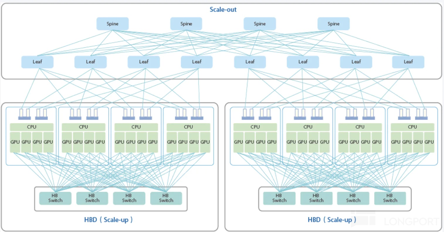
If the destination accelerator is in the same Scale-Up domain, traffic is switched by a proprietary interconnect ASIC and accessed via load/store, i.e., memory semantics. This delivers low latency by bypassing heavy protocol stacks and addressing memory directly.

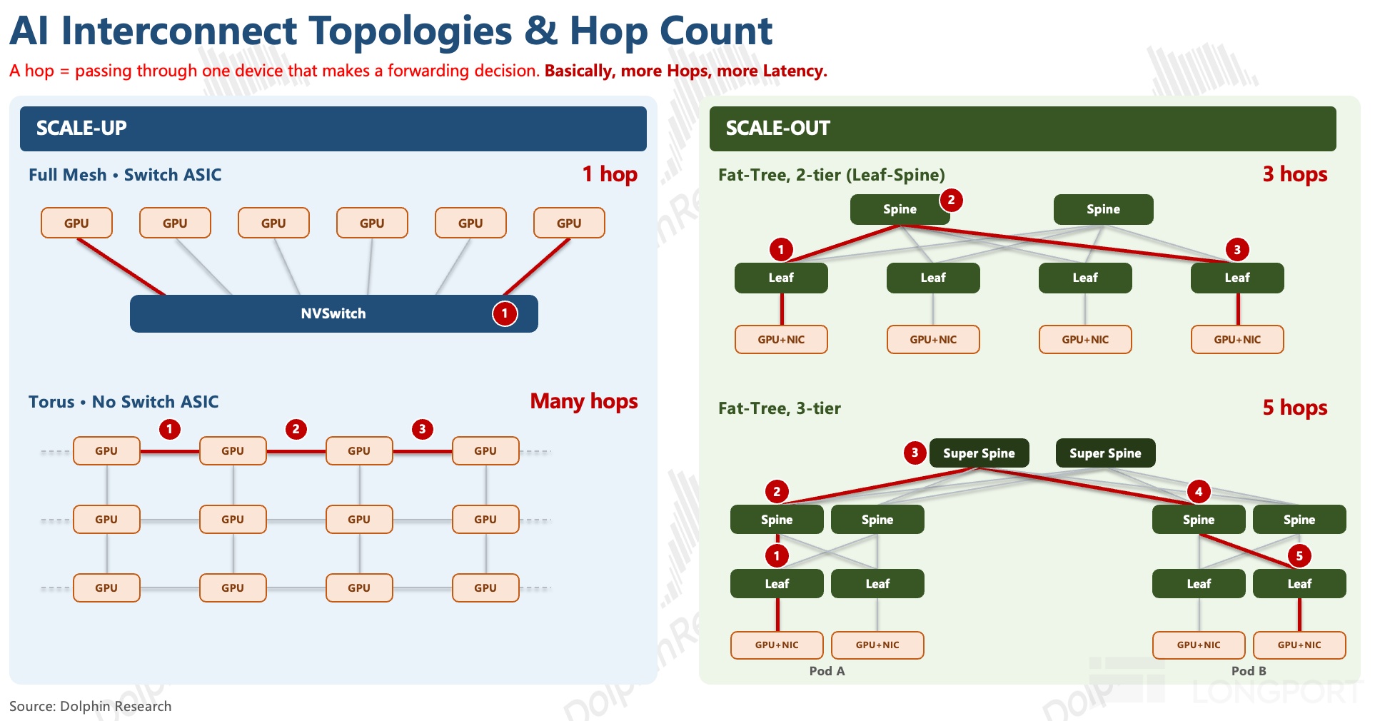
A common metric for path length is hops: each device making a forwarding decision adds one hop, and more hops mean higher latency. With a switch ASIC in the Scale-Up domain, any two GPUs are one hop apart, minimizing path stretch and jitter.

Without a switch ASIC and under direct-connect topologies such as Torus, traffic detours with multiple hops for a given scale. On the Scale-Out side, two-tier fat trees cost 3 hops and three-tier cost 5, as shown below, emphasizing why minimizing hops is a core design goal.

c) Scale-Out

If the destination accelerator sits outside the Scale-Up domain, flows are handed to the NIC/DPU for egress. They pass through electrical interfaces into optical modules, undergo E-to-O conversion, and traverse optical fiber across racks to the next switch tier.

At the switch, O-to-E restores the signal into the ASIC, which makes the next-hop decision and forwards the packet. In multi-tier topologies, traffic progresses through Leaf, Spine, and Super-Spine stages before reaching the target server.

III. The ecosystem battle of interconnects: protocol is the soul

With hardware covered, we turn to protocols. If hardware is the infrastructure, the protocol is the operating rulebook, defining communication semantics, scalability limits, and interoperability. It ultimately governs who can plug into whom at each layer.

Latency and bandwidth requirements differ by layer, and ecosystems form around camps whose standards gain acceptance across peers and the supply chain. Market share of shipped hardware under a standard is the practical scoreboard for strength.

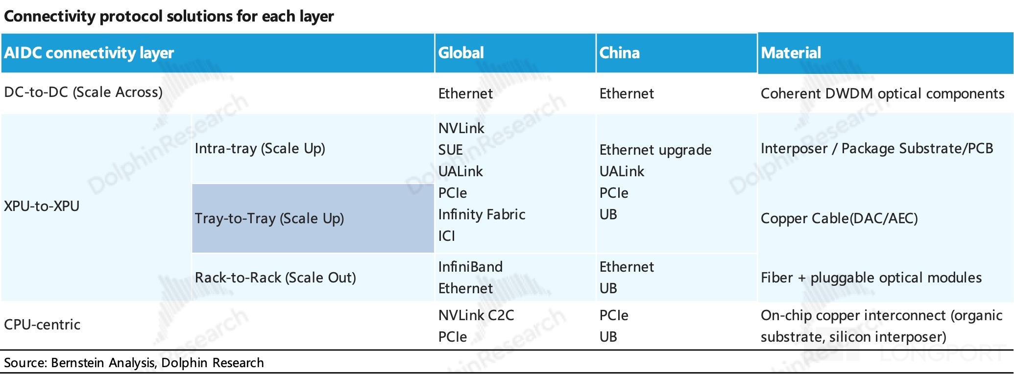
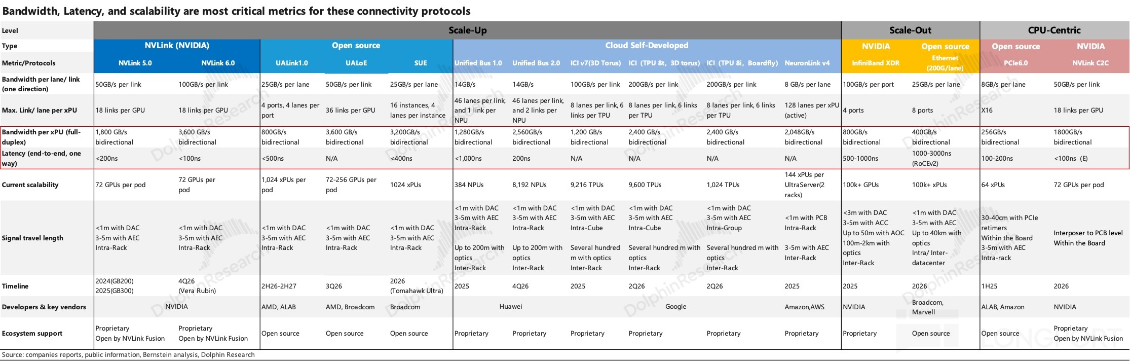
We summarize protocol performance by layer in the tables above, highlighting bandwidth and latency as the critical metrics. These two dimensions define where each protocol excels and where it falls short in practical deployments.

By layer, the epicenter of innovation is the Scale-Up domain, where vendors aim to be the de facto standard setters. Proprietary schemes coexist, including NVIDIA NVLink, AMD UALink, and Huawei UB, each with distinct trade-offs in performance, cost, and ecosystem maturity.

The Scale-Out layer is clearer: the contest is primarily between NVIDIA-led InfiniBand and open-ecosystem Ethernet. Each has strengths by workload and operator preference, often co-existing in large campuses.

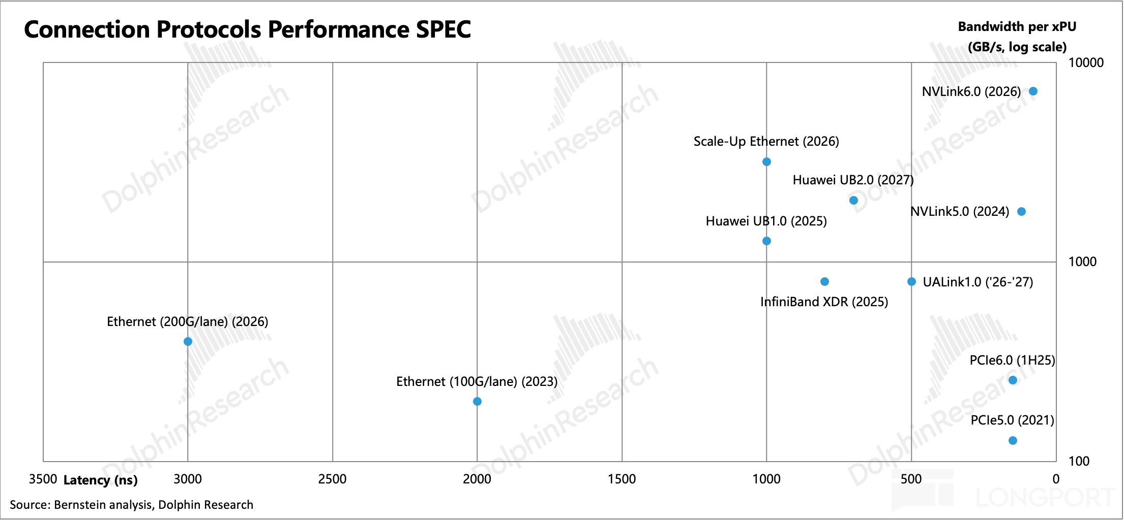
On raw protocol performance, NVIDIA effectively runs parallel closed and open paths and remains the benchmark, with solutions trending toward the top-right of the latency–bandwidth frontier. Yet CSPs still balance performance, budget, and control, enabling open camps like UALink and Broadcom SUE to gain traction.

This primer on network connections ends here. Next, we will dissect differences between AMD and NVIDIA architectures to judge whether Helios can truly challenge NVDA’s GB and VR NVL 72.

<End>

Related Dolphin Research pieces:

Jun 3, 2026: AI in the Ultra-Connected Era: Racing Toward Optics?

Jun 24, 2026: ‘Copper’ Isn’t Leaving: CPO — Real Opportunity or Mirage?

Risk disclosure and disclaimer: Dolphin Research Disclaimer and General Disclosure